Scheduling
Act of selecting the next process/thread to run on the CPU.
Terms
When running, tends to use all the processor time allocated to it. It would go faster if the CPU were faster.
When running, tends to use the processor only briefly before generating an I/O request and relinquishing the processor. It would go faster if the I/O subsystem were faster.
The amount of time to execute a particular process, from submission to complete servicing:
The objective is to minimize turnaround time.
The amount of time from when a process is submitted to the first time it is scheduled. This is an important performance metric for interactive tasks:
The objective is to minimize response time.
The average number of processes (jobs) that complete their execution per unit of time. The objective is to maximize throughput.
All similar processes (jobs) are treated the same. Even if processes are in different priority classes, no process should suffer indefinite postponement (starvation).
Scheduling algorithms
Dispatched according to arrival time.
Example
Based on the above table:
| Time | Queue | CPU |
|---|---|---|
| 0--2 | -- | A |
| 2--3 | B | A |
| 3--4 | -- | B |
| 4--6 | C | B |
| 6--8 | C,D | B |
| 8--9 | C,D,E | B |
| 9--13 | D,E | C |
| 13--18 | E | D |
| 18--20 | -- | E |
The completion times are , , , , and . Therefore, the turnaround times are:
Hence, the average turnaround time is
Dispatched according to the shortest CPU burst time among the processes currently in the ready queue. SJF is non-preemptive, so a process runs to completion once it has been dispatched.
Example
Based on the above table:
| Time | Queue | CPU |
|---|---|---|
| 0--2 | -- | A |
| 2--3 | B | A |
| 3--4 | -- | B |
| 4--6 | C | B |
| 6--8 | C,D | B |
| 8--9 | C,D,E | B |
| 9--11 | C,D | E |
| 11--15 | D | C |
| 15--20 | -- | D |
The completion times are , , , , and . Therefore, the turnaround times are:
Hence, the average turnaround time is
Selects the ready process with the greatest response ratio:
where is the waiting time and is the estimated CPU burst time. HRRN is non-preemptive and reduces starvation by increasing a process's priority as it waits.
Example
For the example table, the schedule is
The turnaround times are , respectively, giving an average turnaround time of
Preemptive scheduling
Running processes may be interrupted and moved to the ready queue, allowing another process to run.
- Preemptive version of SJF
- Arriving processes will trigger scheduler to check against the remaining running time to existing and new processes
- Schedules the process with the shortest run-time-to-completion next
Example
For the example table, the schedule is
The turnaround times are , respectively, giving an average turnaround time of
- Preemptive
- Processes only run for a fixed time quantum (time slice)
- Upon clock interrupt, if current process has its quantum expires, place to the end of the ready queue and schedule the next process in the ready queue
Example
With a time quantum of , the schedule for the example table is
The turnaround times are , respectively, giving an average turnaround time of
Priority scheduling
How it works:
- Consists of a number of queues with priority and a time quantum for each queue
- New job always enters at
- Scheduler always selects a process from the highest priority non-empty
- Within the same queue, processes are scheduled in a round-robin fashion
- If a job at uses an entire (or time allotment), it is demoted to , else, stay at same
- Priority boost: After some time period , move all jobs in the system to
Example
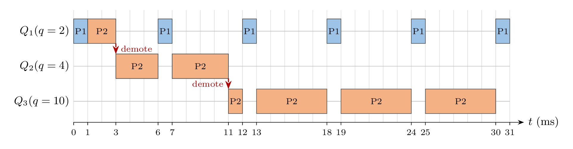
Consider the following scenario in a single-CPU system with two processes, P1 and P2:
- P1 is an interactive process that alternates between CPU and I/O bursts. It runs on the CPU for 1 ms, then performs I/O for 5 ms. This cycle repeats five times, followed by a final CPU burst of 1 ms. The total CPU time required by P1 is therefore 6 ms.
- P2 is a CPU-bound process that runs continuously on the CPU for 30 ms without any I/O.
- At , both P1 and P2 are ready and P1 is ahead of P2 in the queue.
- No priority boost is applied in this scenario.
Caveats of MLFQ:
-
Starvation: A process may never get CPU time if it is always preempted by higher-priority processes.
For example, when a CPU-bound process is running, it may be preempted by a new interactive process that arrives in the system. If this happens repeatedly, the CPU-bound process may never get a chance to run. Solution:
Priority boost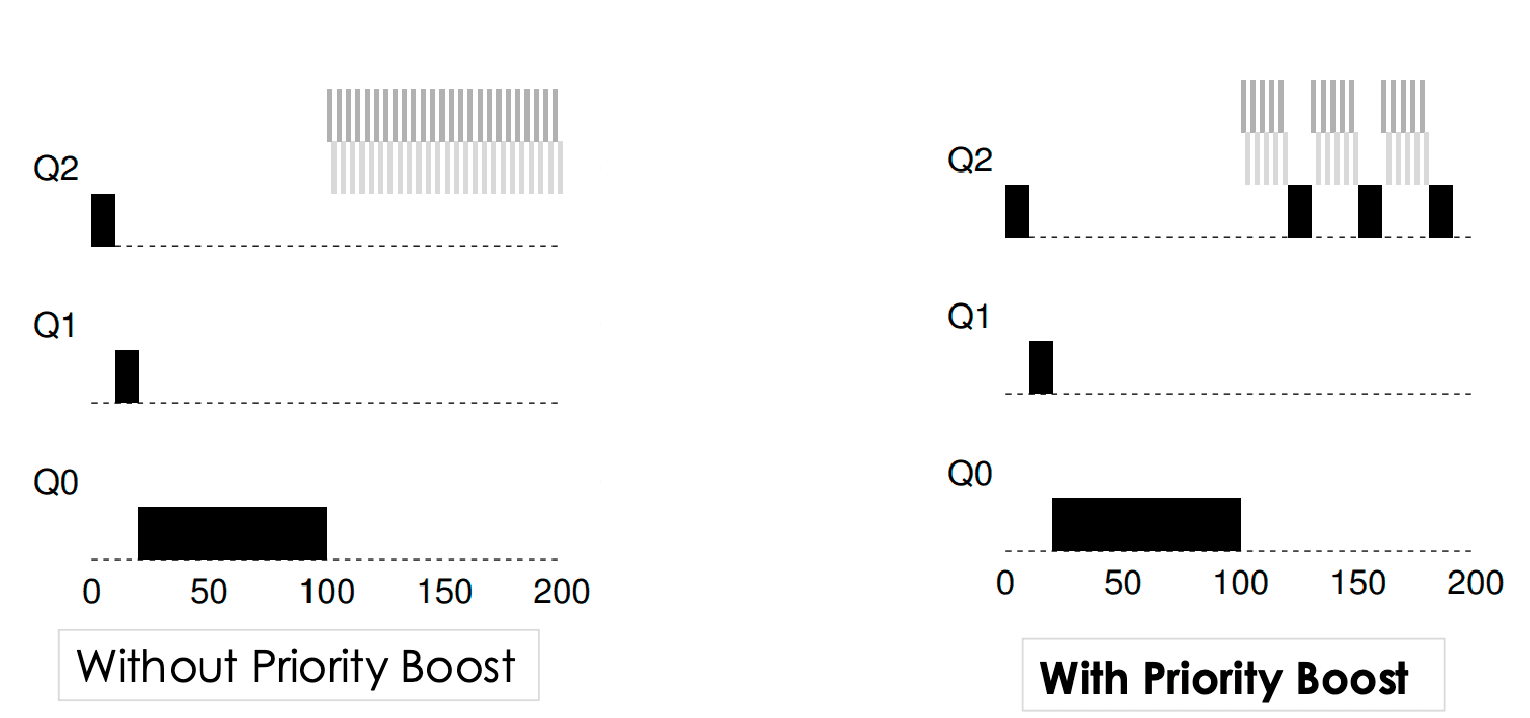
-
Misbehaving processes: A process can end it's CPU burst right before to avoid being demoted. Solution:Time allotment
Keep resource distribution even by considering the process's owner (mother process / user who initiated the process).
Probabilistic fair share scheduling:
- Lottery tickets are distributed to processes, each ticket represents a chance to win the CPU
- To keep fair, a process group/user is given a number of tickets proportional to the resources it is entitled to
- When the scheduler runs, it randomly selects a ticket and the process holding that ticket is given the CPU
- Lottery scheduling is probabilistically fair, meaning that over time, each process will receive CPU time proportional to the number of tickets it holds
Deterministic fair share scheduling:
- Stride = (some number n) / (tickets held by process)
- Each process has a pass value that is initially set to 0.
- CPU picks the process with the lowest pass value to run next.
- After running, the process's pass value is incremented by its stride.