Ranking
Multidimensional data
Many data types are really tables of objects with several attributes, so each object can be expressed as a point in n-dimensional space.
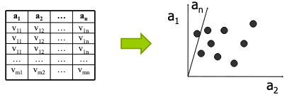
Attributes can be numerical (ordinal) (age, salary), categorical (color), or binary (gender).
Basic queries
- Range query: Find all objects in a given range of values for each attribute.
- Distance query: Find all objects within a given distance
dfrom a reference record. - Nearest neighbor query (kNN): Replaces the distance query's
dbound with a numberkof nearest neighbors to find (ranking)
Top-k queries
Find the k best objects according to an aggregate function f. Attributes values are normalized to [0, 1] to avoid biasing the aggregate function.
Top-k generalizes kNN: kNN ranks by one attribute d, whereas top-k ranks by an aggregate function f of multiple attributes.
Relational table containing inforation about restaurants with attributes price, quality and location.
An example function can be f: sum(-price, quality, -spd(location, my_hotel)), which ranks restaurants by low price, high quality and close location.
- Single table vs. ranked lists: data can be in one table, or sorted lists of each attribute.
- Centralized vs. distributed: lists may sit on one machine or on different servers, and a merger combines them
Most algorithms assumes f is:
- Distributive:
f(x,y,z) = f(f(x,y), z), so partial results can be combined to get the final result (e.g. asumfunction is distributive) - Monotone: if
x >= ythenf(x, z) >= f(y, z), so if a record is worse than another in all attributes, it cannot be in the top-k.
Rank aggregation evaluations
Each attribute has its own ranked list, accessed sequentially and/or randomly.
Pros:
- Works on any subset of attributes
- Suits distributed data
- Easy to implement
Cons:
- Slower than index-based methods
- Needs sorted inputs
Consider multiple ranked lists with values attr[j][i] = (r_ji, v_r) where r_ji is the record and v_r is the value of the attribute j for that record.
TA process the ranked lists row by row. To find the best k records for an aggregate function f with n ranked lists:
- For row
i, computef(r_ji)for eachnlists - Maintain sorted return list
topk[1..k]: rof top-k records - Update threshold
T=f(attr[1][i], ..., attr[n][i])* - Stop when
f(topk[k]) >= T.
*: By monotonicity, any record not yet seen cannot have f(r) > T.
Consider following attr with k=2 and f: sum:
| S1 | S2 | S3 |
|---|---|---|
| c 0.9 | a 0.9 | c 0.9 |
| d 0.8 | b 0.8 | a 0.9 |
| b 0.6 | e 0.6 | b 0.8 |
| e 0.3 | d 0.4 | d 0.6 |
| a 0.1 | c 0.2 | e 0.5 |
Compute:
i | Access | Computed (new) | topk | T | Stop? |
|---|---|---|---|---|---|
| 1 | c, a, c | f(c) = 2.0, f(a) = 1.9 | [c, a] | 0.9+0.9+0.9=2.7 | No (f(topk[2]) = 1.9 < T) |
| 2 | d, b, a | f(d) = 1.8, f(b) = 2.2 | [b, c] | 2.5 | No (f(topk[2]) = 2.0 < T) |
| 3 | b, e, b | f(e) = 1.4 | [b, c] | 2.0 | Yes (f(topk[2]) = 2.0 <= T) |
Returned: [b, c] with f(b) = 2.2, f(c) = 2.0.
NRA also processes the ranked lists row by row, but it never performs random accesses. Since a record's full score is usually unknown, NRA maintains bounds for every record seen so far. To find the best k records for an aggregate function f with n ranked lists:
- For row
i, readattr[j][i]for each of thenlists (sorted access only) - For each record
xseen so far, update the bounds *:lb(x):f(x)with every unseen attribute set to the worst value (0)ub(x):f(x)with every unseen attribute set to the last value seen in that list
- Maintain
W[1..k]: r, thekrecords with the largestlb - Stop when
min lb(W) >= max ub(x)over allxnot inW(an unseen record hasub = f(attr[1][i], ..., attr[n][i])).
*: By monotonicity, the score of x can never exceed ub(x) or fall below lb(x). NRA may stop without knowing the exact score of every record.
Consider following attr with k=2 and f: sum:
| S1 | S2 | S3 |
|---|---|---|
| c 0.9 | a 0.9 | c 0.9 |
| d 0.8 | b 0.8 | a 0.9 |
| b 0.6 | e 0.6 | b 0.8 |
| e 0.3 | d 0.4 | d 0.6 |
| a 0.1 | c 0.2 | e 0.5 |
Compute (bounds are [lb, ub]):
i | Access | Bounds (seen records) | W | Stop? |
|---|---|---|---|---|
| 1 | c, a, c | c [1.8, 2.7], a [0.9, 2.7] | [c, a] | No (min lb(W) = 0.9 < 2.7, unseen records have ub = 2.7) |
| 2 | d, b, a | c [1.8, 2.6], a [1.8, 2.6], d [0.8, 2.5], b [0.8, 2.5] | [c, a] | No (1.8 < ub(d) = 2.5) |
| 3 | b, e, b | b 2.2, c [1.8, 2.4], a [1.8, 2.4], d [0.8, 2.2], e [0.6, 2.0] | [b, c] | No (1.8 < ub(a) = 2.4) |
| 4 | e, d, d | b 2.2, c [1.8, 2.2], a [1.8, 2.1], d 1.8, e [0.9, 1.5] | [b, c] | No (1.8 < ub(a) = 2.1) |
| 5 | a, c, e | b 2.2, c 2.0, a 1.9, d 1.8, e 1.4 | [b, c] | Yes (min lb(W) = 2.0 >= ub(a) = 1.9) |
Returned: [b, c] (ties between lbs broken arbitrarily), with f(b) = 2.2, f(c) = 2.0.
| TA | NRA | |
|---|---|---|
| Access types | Sorted and random | Sorted only |
| Stopping rule | k-th best score ≥ T | min lb in ≥ max ub outside |
| Scores | Exact for each seen object | Bounds, possibly never exact |
| Overhead | Costly random accesses | Bound storage for all seen objects |
| Best when | Random access is cheap | Random access is costly or impossible |